Complete male fruit fly connectome: inside the 166,700-neuron map

The milestone in one sentence

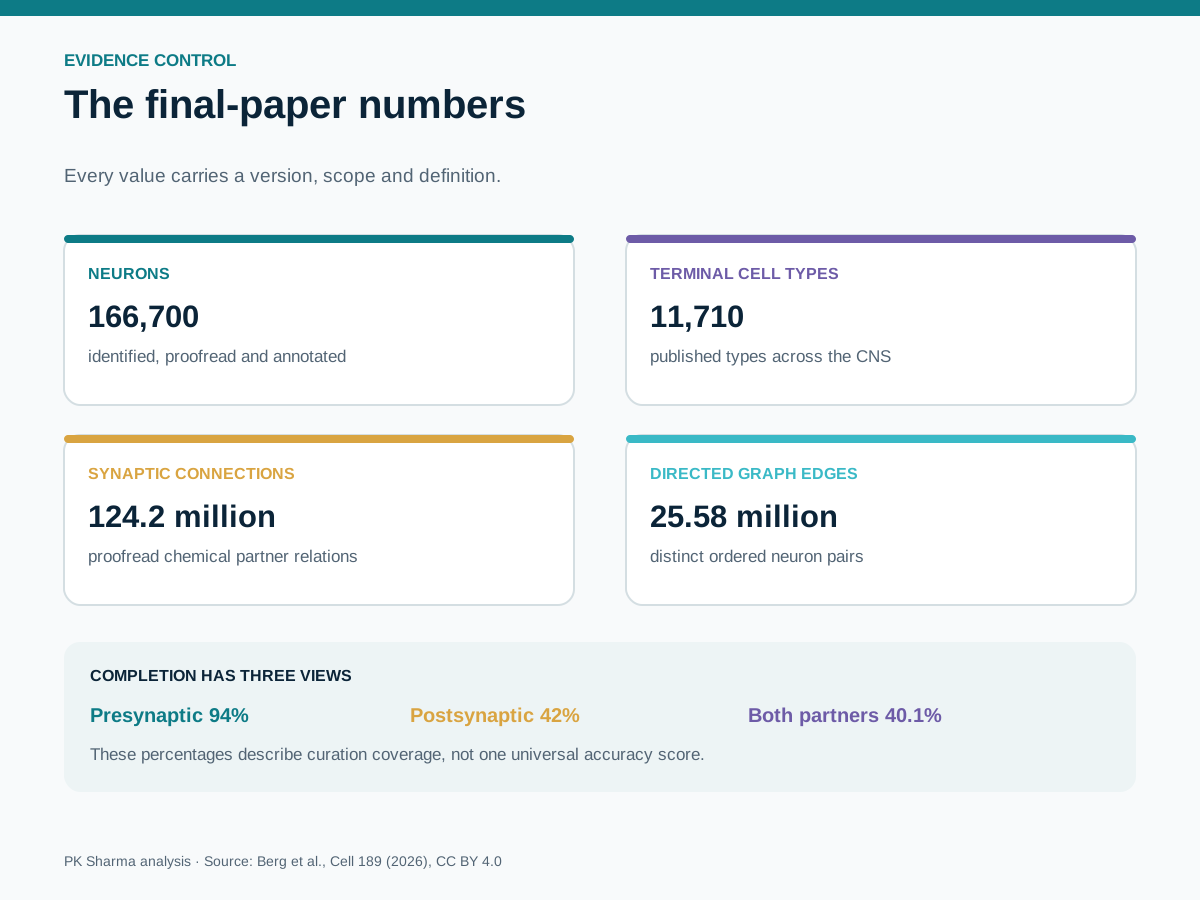
Scientists have released the first synapse-level wiring diagram that spans the entire central nervous system of an adult male fruit fly: the brain plus the ventral nerve cord that controls much of the body. The final peer-reviewed dataset contains 166,700 reconstructed neurons, organised into 11,710 terminal cell types, with 124.2 million proofread synaptic connections. When those synapses are collapsed into a graph, they form 25.58 million directed edges among 166,483 connected neurons; another 217 reconstructed neurons have no retained graph connection under the release criteria.

That combination matters more than any one number. Earlier atlases mapped major parts of the fly brain, and other studies mapped circuits or smaller animals, but this resource makes it possible to follow pathways across the adult male fly's brain and nerve cord in one coordinate system. A researcher can start at a sensory neuron, trace candidate partners, move through interneurons and descend into motor pathways without crossing between independently reconstructed specimens.

The release is a platform as well as a paper. Its value comes from the alignment of image evidence, three-dimensional reconstructions, synaptic partners, cell identities and public query tools. A numerical claim can be followed back toward the cells that produced it. A proposed circuit can be inspected spatially and converted into an experimental shortlist. That audit path is what turns an impressive image volume into shared scientific infrastructure.

The achievement is also easy to overstate. A connectome is a structural map, not a recording of thought, a complete simulation or a catalogue of every molecule. It provides the wiring on which hypotheses can be built. Activity, neuromodulation, learning, internal state and the physics of the body still have to be measured.

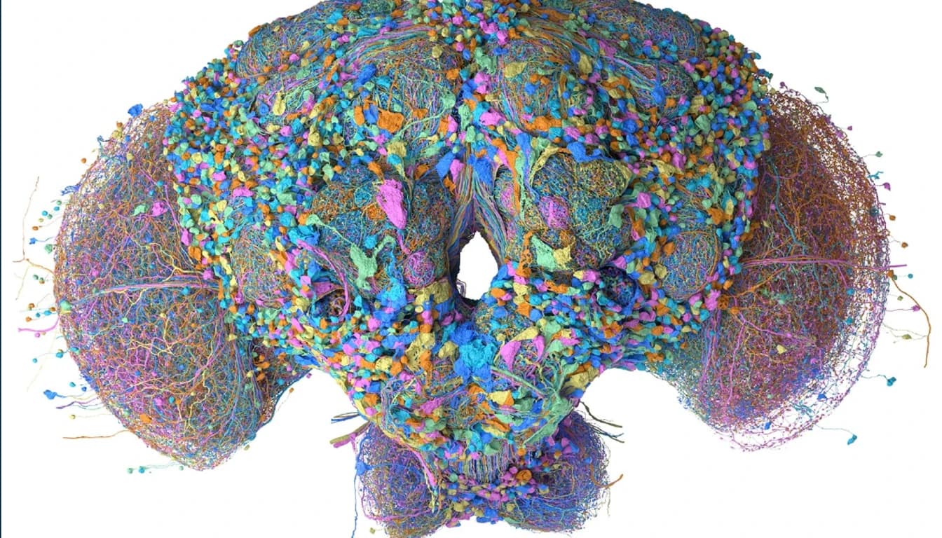
Hero image: HHMI Janelia FlyEM Project Team, Cambridge and MRC LMB collaborators, and Google Research. Source: MaleCNS Connectome Project v1.0; CC BY.

What complete means, and what it does not

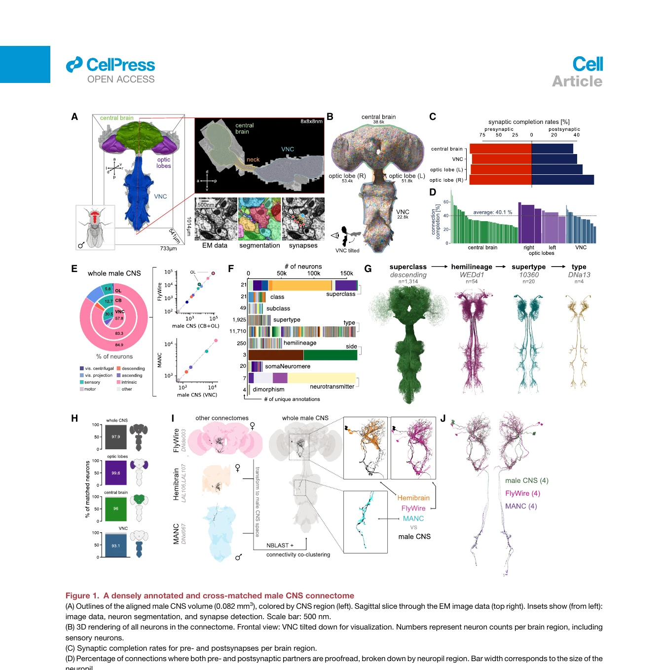
In connectomics, the word complete needs a scope. Here it means the electron-microscopy volume covers the central nervous system of one adult male specimen, including brain and ventral nerve cord, and the team attempted to reconstruct and annotate the neurons within that volume. It does not mean every synapse has equal certainty or that every neurite is perfectly traced.

The final paper reports that 94 percent of presynaptic sites and 42 percent of postsynaptic sites are connected to proofread neuronal reconstructions. Considering both sides together, 40.1 percent of synaptic connections have proofread partners on both ends. These values describe a huge, highly curated resource while making the residual incompleteness visible.

Coverage, tracing and synaptic assignment are separate dimensions. A volume may contain a neuron whose thin branch is difficult to follow. A traced neuron may reach the edge of the imaged tissue. A putative contact may be detected automatically but fail a confidence threshold. Treating all three dimensions as one percentage hides the actual uncertainty.

A disciplined reading of completeness

Layer	What the release provides	What remains outside the claim
Anatomical coverage	One adult male central nervous system, brain and ventral nerve cord	Peripheral organs, most muscles and other individual flies
Neuron reconstruction	166,700 reconstructed neurons with extensive proofreading	Some unresolved fragments, fine branches and boundary effects
Synapse graph	124.2 million proofread synaptic connections and 25.58 million directed edges	A graph edge does not by itself establish functional influence
Cell identity	11,710 terminal cell types linked to annotations and cross-sex matches	Cell-state variation and every possible molecular subtype
Behaviour	Structural routes associated with sensory, motor and social functions	Real-time dynamics, intention, memory content or a full behavioural simulator

How to read the headline numbers without losing the science

Large numbers make the release legible to a general audience, but each one answers a different question. The neuron count describes reconstructed cellular objects included in the final atlas. It is not a count of independent computational units in the engineering sense: neurons differ enormously in size, branching, chemistry, partners and role.

The 11,710 terminal cell types are annotation categories, not 11,710 behaviours. Some types contain many repeated neurons; others may have very few members. A type expresses a judgement that cells share enough anatomy and connectivity to belong together. That judgement becomes stronger when it survives comparison across hemispheres, sexes or specimens.

The 124.2 million proofread synaptic connections describe directed contacts assigned within the curated reconstruction. The term connection at this level can refer to an individual presynaptic-to-postsynaptic relation. The 25.58 million graph edges instead count distinct ordered neuron pairs after contacts between the same pair are grouped. Reporting both prevents a common category error in which synapses and edges are compared as if they were the same unit.

Counts also depend on inclusion rules. Tiny disconnected fragments, cells that extend beyond the imaged volume and uncertain contacts can be retained, excluded or reported separately. The final article notes 166,483 neurons in the connected graph and 217 reconstructed neurons without a retained connection, which together reconcile with the headline total of 166,700. Without that reconciliation, a reader could wrongly conclude that the paper contradicts itself.

Proofreading percentages describe coverage of the synaptic evidence, not a universal accuracy score. The high presynaptic coverage reflects how the reconstruction was prioritised and how output sites are used to identify partners. Lower postsynaptic coverage means many input sides still involve unproofread material. The 40.1 percent figure for connections with both partners proofread is the strictest of the reported completeness views.

Finally, the 160-teravoxel image volume describes the scale of the raw three-dimensional evidence. It cannot be converted directly into neuron count or biological complexity. Voxel size determines what structures can be resolved; tissue preparation, imaging quality and alignment determine whether that resolution is usable. These distinctions are why the report keeps a claim ledger instead of presenting one giant number as a proxy for the entire achievement.

One release, several units

Number	Unit	Question it answers
166,700	Reconstructed neurons	How many cellular objects are represented in the final atlas?
11,710	Terminal cell types	How finely does the published taxonomy organise those neurons?
124.2 million	Proofread synaptic connections	How many directed synaptic partner relations are retained?
25.58 million	Distinct directed graph edges	How many ordered neuron pairs are connected after grouping contacts?
160 teravoxels	Image-volume samples	How large is the aligned electron-microscopy evidence base?

From one specimen to 160 teravoxels

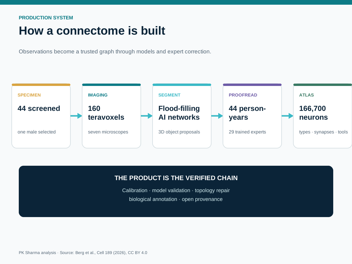
The atlas began with physical tissue, not a graph. The nervous system was fixed, stained with heavy metals, embedded, cut into ultrathin sections and imaged by electron microscopy. The resulting volume contained roughly 160 teravoxels at 8 by 8 by 8 nanometre voxels. Seven microscopes collected the material over about thirteen months.

At that scale, manual tracing from blank images would be impractical. Machine-learning models first identified cellular boundaries and synaptic sites. Segmentation joined voxels into candidate neuronal objects. Automated proposals were then checked, corrected and merged by expert proofreaders. Annotation teams assigned anatomical names, cell classes, transmitter predictions and cell types. The graph used for analysis was built only after those stages.

Each transformation can introduce a different error. A missing section affects imagery; an incorrect boundary affects segmentation; a false merge can join two neurons; a false split can divide one neuron; a missed synapse changes an edge; and a wrong type label affects every analysis grouped by that type. The release is valuable because these layers remain inspectable rather than being compressed into an unexplained network file.

The AI systems and the human correction bottleneck

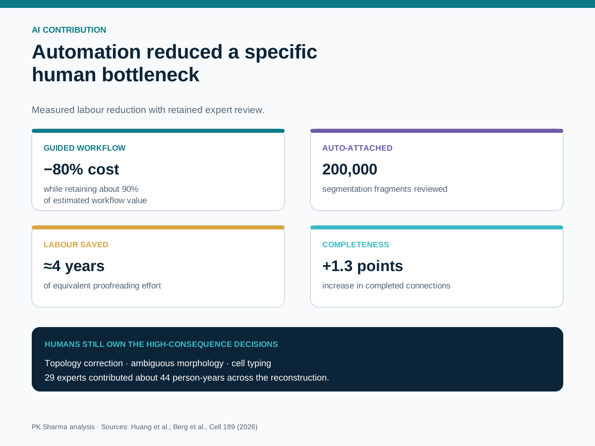
The reconstruction pipeline combines specialised models rather than one general-purpose AI. Flood-filling networks helped produce dense neuronal segmentation. Separate systems detected synapses and predicted neurotransmitters from local electron-microscopy context. Human experts then reviewed the structures with tools designed to surface likely errors.

That last stage has historically dominated the cost. AutoProof addresses it by ranking and proposing corrections for suspicious regions. Google reports that the system recovered about 90 percent of the value of a guided proofreading workflow at 80 percent lower cost. Applied to roughly 200,000 fragments, the process represented about four proofreader-years and improved the percentage of proofread synaptic connections by around 1.3 points.

Those figures should be read precisely. AutoProof does not generate the whole connectome from raw tissue, and an efficiency gain is not the same as an error-free result. It narrows the expensive human search problem: experts spend more time judging likely faults and less time scanning everything uniformly. This pattern is likely to matter across scientific AI, where the strongest systems often allocate expert attention rather than eliminate it.

The resource is a stack, not one enormous file

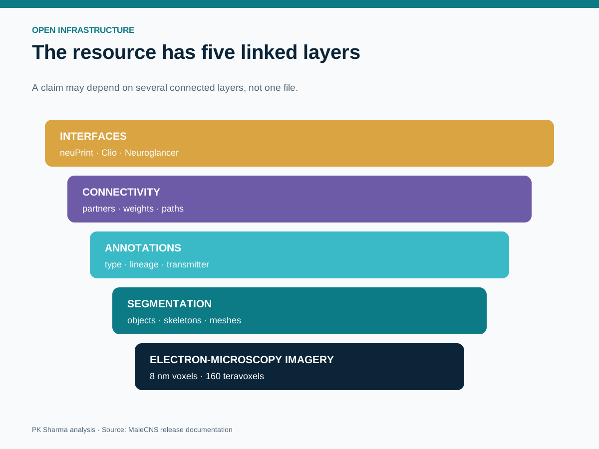
The public release is designed for several kinds of work. Neuroglancer supports spatial inspection of image volumes and reconstructions. Codex provides cell search, connectivity tables and annotations. NeuPrint exposes graph-oriented queries. Download packages and supplemental repositories support reproducible analysis in local code.

The useful mental model has five layers. Raw and aligned imagery preserves the evidence. Segmentation turns the imagery into three-dimensional objects. Synapse tables connect presynaptic and postsynaptic sites. Annotation tables attach identities, types, regions and predictions. Graph interfaces convert those records into queries about partners, paths, motifs and communities.

Researchers must keep identifiers and release versions together. A cell identifier without the dataset version can become ambiguous after corrections. A graph statistic without the edge threshold may not reproduce. A figure without its query and software environment may look authoritative while being impossible to audit.

Four common interfaces and the jobs they serve

Interface	Best use	Audit record to save
Neuroglancer	Inspect morphology, image evidence and spatial relationships	Dataset version, coordinates, layers and screenshot context
Codex	Find cells by type or annotation and review partners	Cell IDs, filters, sorting and export date
NeuPrint	Run graph queries and aggregate connectivity	Query text, server dataset, thresholds and returned IDs
Bulk downloads	Reproduce analyses, build models and join tables	File names, hashes, release notes and analysis environment

What a researcher can ask now

The atlas turns anatomical questions into inspectable graph operations. Suppose a team studies how an odour can alter locomotion. It can identify olfactory input types, rank their strongest downstream partners, find paths into descending neurons, inspect whether the candidate cells project into the ventral nerve cord, and compare the resulting circuit with behavioural experiments.

Another team might begin with a motor output. Starting from neck or leg motor neurons, it can trace upstream interneurons and descending pathways to ask which brain regions converge on that action. The result is not proof that a particular route causes the behaviour. It is a constrained list of candidates and junctions that can be tested with genetics, imaging or electrophysiology.

The full central nervous system changes the scale of those questions. Previous brain-only maps could end at a descending neuron. This resource lets a query continue through the cord toward motor systems. It therefore closes an anatomical gap between decision-related circuits and body control.

Examples of answerable questions

Starting point	Graph operation	Experimental follow-up
A sensory cell type	Rank partners and trace paths to descending neurons	Silence or activate selected intermediates
A motor neuron	Walk upstream and locate convergent control pathways	Record activity during the corresponding movement
A cell type shared across sexes	Compare counts, morphology and connection weights	Test whether structural differences predict behaviour
A transmitter prediction	Group outputs by predicted chemical identity	Validate markers or pharmacological response
A recurrent motif	Measure loops, hubs and alternative paths	Perturb nodes to test robustness and compensation

The male–female comparison changes the scientific question

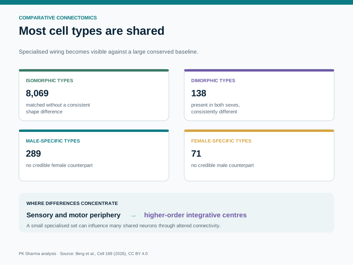
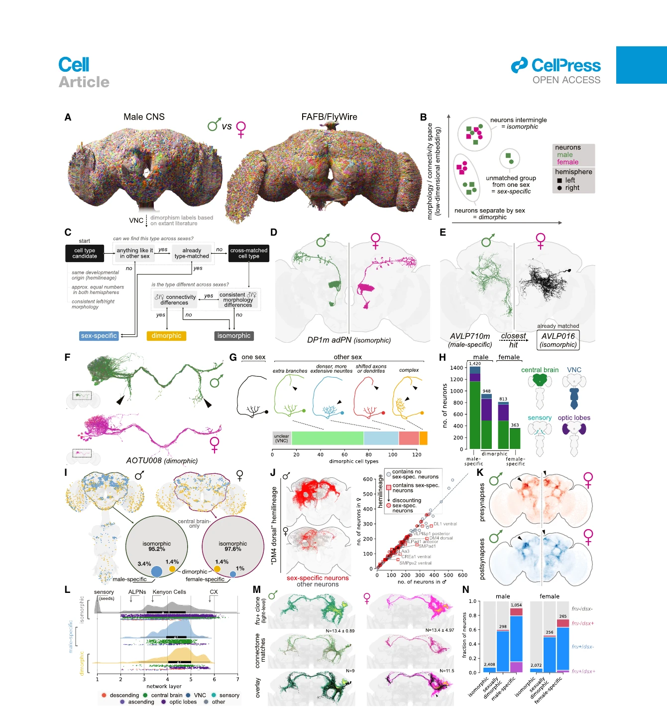
The male map becomes more informative when aligned with the female adult nerve-cord and brain connectome. The final analysis identifies 8,069 isomorphic cell types that can be matched across the sexes, 138 sexually dimorphic types, 289 male-specific types and 71 female-specific types.

The largest category is conserved. That is scientifically useful because it provides a structural baseline for locomotion, sensation and core computation. The smaller sex-linked categories then stand out against that baseline. Dimorphism can appear as a difference in cell number, morphology, connection strength or partner choice. A sex-specific type is a stronger claim: the matching procedure finds a type in one atlas without an equivalent in the other under the stated criteria.

These counts do not say that every behavioural sex difference is hard-wired or that all individuals share identical wiring. Each whole-volume atlas still represents one specimen. The comparison reveals candidate structural mechanisms and makes the definitions explicit enough to test in more animals.

Vision, taste and social behaviour are already becoming test cases

A connectome earns its value through analyses that expose organising principles. Companion studies use the same release to examine visual pathways, gustatory circuits and sexually dimorphic social-behaviour networks.

The visual analysis follows parallel channels from the optic lobes into central circuits. It shows how information is routed through hierarchical and recurrent pathways rather than a single feed-forward ladder. For machine vision, the relevant lesson is architectural: biological perception uses specialised channels, feedback and task-linked compression. The map does not supply a ready-made neural-network blueprint.

The gustatory study connects receptor classes to feeding, foraging and social circuits. Taste is a good demonstration because the signal is not merely labelled sweet or bitter; its influence depends on internal state, action selection and interactions with other senses. The structural graph helps locate where these influences may converge.

The social-behaviour study identifies networks of sexually dimorphic neurons associated with courtship and aggression. Its strongest contribution is a testable circuit framework. It narrows the space of candidate cells and connections while leaving causal claims to targeted perturbation and measurement.

One atlas, several scientific programmes

Programme	Structural question	What the map cannot decide alone
Vision	How parallel sensory channels converge, recur and reach action pathways	What a neuron represents in a live task
Taste	How receptor inputs reach feeding, foraging and social circuits	How hunger and learning change moment-to-moment gain
Social behaviour	Which conserved and sex-linked pathways connect sensory cues to action	Whether a connection is necessary or sufficient for behaviour
Motor control	How brain commands continue through descending and cord circuits	The mechanics and feedback of the behaving body

Why including the ventral nerve cord changes the map

The adult fly central nervous system has two major connected domains. The brain contains optic lobes, central sensory-processing regions, association areas and centres involved in navigation, memory and action selection. The ventral nerve cord contains dense premotor and motor circuitry for the legs, wings, neck and abdomen. Descending neurons carry signals from brain to cord; ascending neurons return sensory and state information.

A brain-only atlas can identify a candidate descending command but may stop before the signal reaches the circuits that coordinate joints and muscles. A cord-only atlas can reveal local motor organisation but may not show how visual, olfactory or internal-state pathways selected the action. The male CNS volume puts those domains into one specimen and one geometric frame.

This matters for apparently simple behaviour. Turning toward an odour can require olfactory classification, comparison across time, integration with hunger or courtship state, selection of a direction, descending control and coordinated leg movements. Flight adds visual stabilisation, wing steering and rapid feedback. Grooming recruits a different hierarchy in which stimulation of one body region can suppress or reorder another movement. A path across brain and cord lets researchers see where these streams may converge and compete.

The resource also captures ascending routes. Motor control is not a one-way broadcast from a brain to passive limbs. Sensory neurons and interneurons report contact, position and movement. Those signals can reshape ongoing action within the cord or travel upward. The complete CNS scope therefore supports questions about closed loops, even though the connectome itself is a static snapshot of their structure.

How 124.2 million synapses become a 25.58-million-edge graph

A synapse table and a neuron graph describe related but different objects. Each detected chemical synapse has a location, a presynaptic partner and one or more postsynaptic relationships. Many synapses can connect the same ordered pair of neurons. Graph construction collapses those repeated contacts into a directed edge whose weight is usually the number of contributing synaptic connections.

That is why 124.2 million synaptic connections can yield 25.58 million directed edges. The edge count is lower because several contacts between the same source and target are represented once with a larger weight. Analysts may then apply a threshold, for example retaining only pairs supported by several synapses, to reduce the influence of isolated detections. Every threshold changes reachability, degree distributions and apparent hubs.

Direction carries a limited anatomical meaning: the edge runs from the presynaptic cell toward the postsynaptic cell. It does not guarantee excitation, because the physiological sign depends on transmitter and receptor. It does not guarantee that a connection is active in a particular state. Nor does a large synapse count translate linearly into behavioural importance; a strategically placed weak input can gate a circuit, while many contacts may be redundant.

Cell-type graphs compress the data again. All neurons assigned to one type can be grouped, turning an enormous cell-level network into a more interpretable map of type-to-type connectivity. This is useful for comparison, but aggregation can hide rare cells, left-right asymmetry and individual variation. Strong analysis moves between scales: discover a pattern in the type graph, inspect the contributing cells, then return to imagery where the claim is sensitive to reconstruction quality.

Four representations of the same connectome

Representation	Unit	Best question	Common mistake
Synapse table	Individual directed contact	Where are contacts and which cells participate?	Treating every detection as equally certain
Cell graph	Neuron-to-neuron edge with a weight	Which cells are partners, hubs or paths?	Forgetting the chosen edge threshold
Type graph	Aggregated cell-type connection	Which circuit classes organise the network?	Hiding rare or asymmetric members
Region graph	Connectivity between anatomical areas	How do large systems exchange information?	Inferring a precise cellular mechanism from a coarse flow

From object IDs to biological identity

Segmentation produces objects; neuroscience requires identities. The annotation programme links reconstructed cells to anatomy, morphology, lineage-informed groupings, predicted transmitter and connectivity. Terminal cell types are the most specific published categories in a hierarchy that also includes broader classes and families.

Type assignment is difficult because similar shape does not always imply the same function, and two cells can share a role while differing in fine morphology. Connectivity provides an additional fingerprint: a cell's major inputs and outputs can distinguish otherwise similar structures. Cross-dataset matching adds another constraint by asking whether a candidate type has a plausible counterpart in the female atlas or earlier brain datasets.

This creates a powerful catalogue, but the labels are not timeless facts. As more specimens arrive, some types may split, merge or be redefined. A terminal type with one observed member may prove rare, sex-specific or simply undersampled. A type present in both sexes may vary in abundance or wiring. Reproducible work should therefore carry both immutable cell identifiers and the annotation version used to interpret them.

Predicted neurotransmitters add chemical context. Image-based models can classify likely transmitter identity from synaptic ultrastructure and surrounding features. These predictions help distinguish candidate excitatory, inhibitory and modulatory routes, but receptor expression on the target is also required to infer sign. The honest chain is prediction, supporting evidence, experimental validation and then mechanism.

Where error can enter, and how to contain it

A flagship connectome needs a threat model for scientific error. Imaging artefacts can obscure membranes or synapses. Alignment can distort a boundary between sections. Segmentation can split one neuron or merge two. Proofreading can miss a subtle branch. Synapse detection can omit weak contacts or assign the wrong partner. Annotation can attach a correct morphology to the wrong type. Analysis code can then amplify any of these faults through aggregation.

The controls differ by layer. Imaging problems require inspection of the underlying volume. Segmentation faults require targeted proofreading and comparison with morphology. Synapse claims benefit from confidence scores and local image review. Annotation disputes require explicit definitions and cross-dataset evidence. Analytical errors require versioned queries, tests and independent reproduction.

Scale makes random spot checking inadequate. Quality assurance should be risk-based. A suspected false merge in a highly connected descending neuron matters more to a whole-network conclusion than an uncertain terminal twig in an isolated fragment. A cell used as the sole evidence for a new sex-specific type deserves deeper review than one member of a large conserved family. The dataset's open interfaces allow downstream teams to inspect those high-impact claims.

Derived machine-learning datasets need the same care. Training examples should preserve release identifiers and avoid leakage through bilateral homologues or near-duplicate types. Labels predicted by one model should not quietly become ground truth for evaluating a second model. Reported performance should state whether the split tests new cells, new types, new regions or a genuinely separate specimen.

Error propagation and the matching control

Stage	Failure example	Control
Imaging	Missing or distorted local evidence	Return to aligned sections and document affected regions
Segmentation	False merge or false split	Prioritised proofreading with morphology and partner checks
Synapses	Missed contact or wrong partner	Confidence thresholds and local image validation
Annotation	Incorrect type or transmitter label	Versioned definitions and orthogonal evidence
Analysis	Threshold-dependent result presented as universal	Sensitivity analysis and published query parameters

A connectome is structure, not a running brain

A wiring diagram constrains what a nervous system can do, but it does not specify every state the system can occupy. Synapse count is often used as a proxy for connection strength, yet release probability, receptor composition, neuromodulation and recent activity all affect function. Gap junctions, hormones and volume transmission add interactions that are not fully represented by a directed chemical-synapse graph.

The atlas also freezes one individual at one moment in an invasive preparation. Development, age, experience, injury and natural variation can alter structure. Cell-type labels simplify a continuum of states. Predicted neurotransmitters are powerful annotations, but predictions need independent validation when the conclusion depends on chemical identity.

For simulation, these omissions matter. A graph can support spreading-activation models, motif discovery and constrained dynamical experiments. Calling such a model a digital fly brain would imply far more: validated cellular dynamics, sensory transduction, muscles, biomechanics, learning rules and an environment. The responsible description is a connectome-constrained model.

Could this be used badly? A realistic dual-use assessment

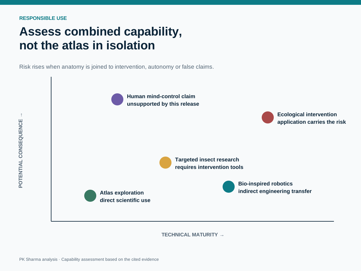
Open biological maps deserve serious risk analysis, but the analysis should follow demonstrated capability. The near-term value of this dataset is scientific: circuit discovery, comparative anatomy, algorithm development and better planning of experiments. It does not provide a recipe for controlling people, reading thoughts or reproducing a human brain.

The most credible immediate risks concern the research system around the data. A corrupted mirror, altered annotation table or model trained on mismatched releases can produce plausible but false conclusions. Selective presentation can turn exploratory graph patterns into exaggerated claims about sex, intelligence or behaviour. Provenance loss can make a derived dataset impossible to audit.

A second category is plausible but indirect. Better understanding of compact sensorimotor circuits may inform small autonomous systems, optimisation methods or bio-inspired control. The connectome is only one input among many, and translating it into a robust engineered system requires dynamics, hardware, objectives and extensive validation. The risk belongs to the application programme, not to a downloadable edge list by itself.

More dramatic scenarios remain speculative. The fly atlas does not enable remote behavioural control, reconstruction of personal memories or direct modelling of human cognition. Treating those claims as current capability distracts from the controls actually needed now.

Controls matched to the actual risk

Risk	Practical control	Why it helps
Dataset tampering	Publish hashes, immutable releases and signed provenance	Users can verify that files match the cited release
Silent version mixing	Pin dataset, schema, code and query versions	Counts and identifiers remain reproducible
Misleading behavioural claims	Separate structure, prediction and causal evidence	Readers can see where inference begins
Sensitive downstream engineering	Review the application, deployment environment and operators	Controls follow the capability that can create harm
Loss of public trust	Keep limitations and corrections visible	Scientific uncertainty becomes part of the product

What bio-inspired AI can learn, and what it cannot copy

The map offers useful design patterns for AI researchers: sparse specialised pathways, recurrence, bilateral organisation, convergent control, modular sensory channels and circuits that link perception to action with a compact energy budget. These patterns can inspire experiments in efficient robotics, continual adaptation and interpretable control.

Copying the adjacency matrix is unlikely to reproduce the animal. Biological computation depends on cell dynamics, synapse types, receptor distributions, neuromodulators, plasticity and embodiment. Even a perfectly reconstructed graph would still need parameters and learning rules that the connectome does not contain.

The strongest engineering method is therefore comparative. Form a hypothesis from a circuit motif, implement several abstracted variants, test them against explicit baselines and report where the biological constraint helped. This approach respects the source while producing evidence that can stand independently of biological metaphor.

The roadmap runs through comparison and function

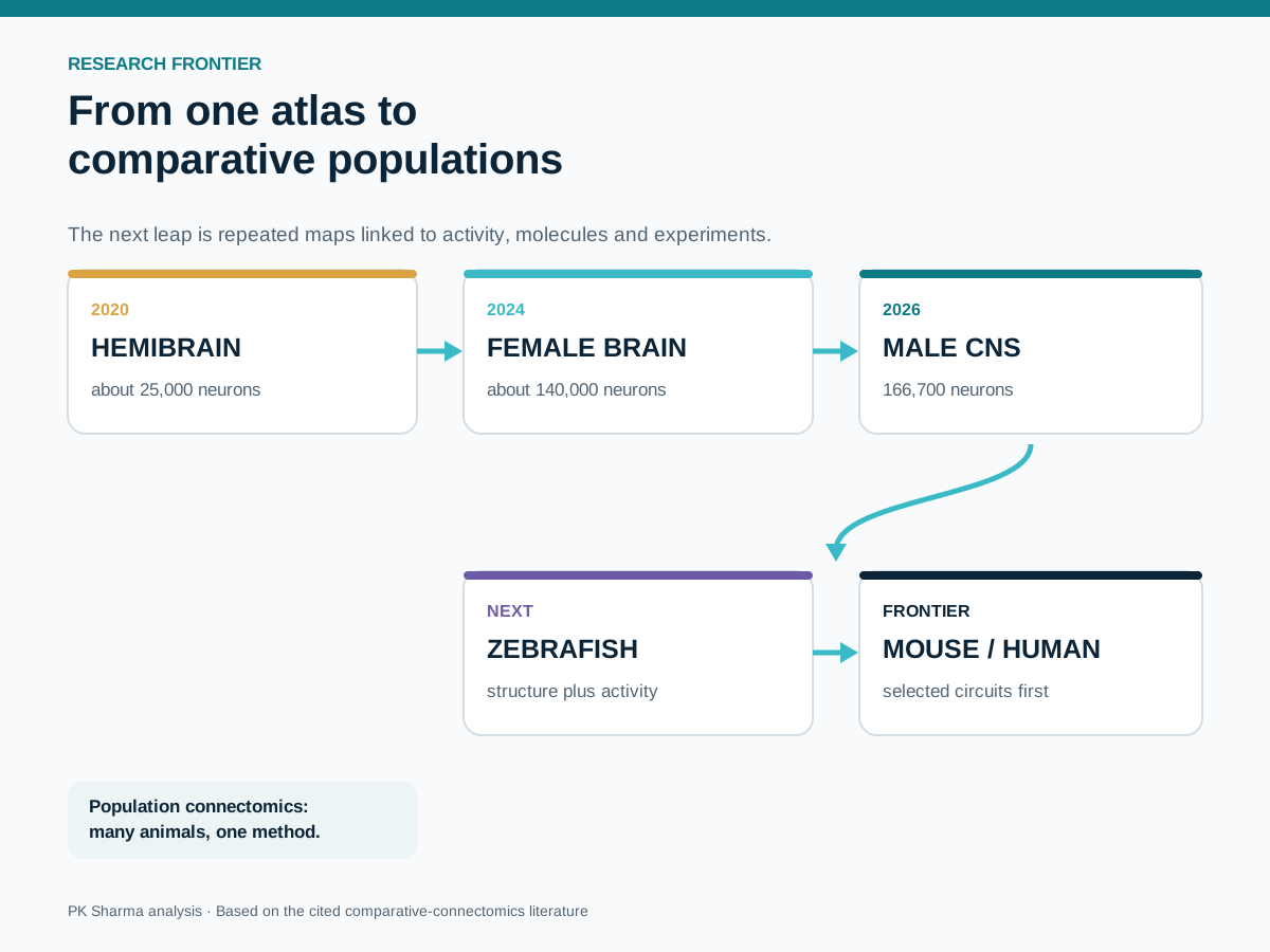
The durable next step is not simply a larger graph. It is a family of comparable, versioned atlases linked to function. The female brain-and-cord connectome already makes cross-sex analysis possible. Additional male and female specimens would reveal which motifs are stable and which vary between individuals. Developmental stages, genetic backgrounds and experience could then be compared with the same discipline.

Other species change the engineering problem. Larger nervous systems demand better automated segmentation, proofreading and cell typing. Vertebrate circuit maps will often be partial or region-focused for some time. Their value will depend on linking structure to activity, molecular identity and behaviour rather than chasing neuron count alone.

The MaleCNS project is therefore both a biological atlas and a production benchmark. It shows that petascale imaging, specialised AI, expert correction and open data interfaces can be assembled into a reproducible scientific resource. The tools and quality controls may travel further than any individual fly circuit.

A minimum reproducibility record

A useful analysis record should answer six questions. Which release was used? Which files or server dataset supplied the data? Which cell identifiers and annotations defined the population? Which thresholds transformed synapses into graph edges? Which query or code produced the result? Which software environment rendered the figure?

Save exact exports and checksums where permitted. Record access dates for live interfaces. Keep intermediate tables that map cell identifiers to labels, because annotation tables can change independently of analysis code. If a result depends on a manually selected set of cells, publish that set as data rather than only naming it in prose.

For cross-sex work, retain the matching table and the definition of isomorphic, dimorphic and sex-specific types. For graph comparisons, normalise deliberately: raw synapse counts, connection fractions and thresholded binary edges answer different questions. For model training, split data in a way that prevents near-duplicate cell types or bilateral homologues from leaking between train and test sets.

Six fields that make a result inspectable

Field	Example record
Release	MaleCNS v1.0 and publication correction status
Source	NeuPrint dataset name or downloaded archive with SHA-256
Selection	Cell IDs, type labels, regions and inclusion rules
Graph rule	Minimum synapse count, direction and weighting
Method	Query text, notebook commit and random seed
Output	Tables, figure data, software versions and provenance

Download the full 85-page research edition

The expanded report carries the evidence in a format designed for slower reading and citation. It includes the construction pipeline, data architecture, cell-type comparison, companion science, AI methods, dual-use analysis, reproducibility checklist, source register and full-size figures from the open-access Cell paper.

The report distinguishes observed facts from interpretation, carries image credits beside reused figures and preserves the final paper as the canonical numerical source. Use the web briefing for navigation and the PDF when you need the full tables, diagrams and audit trail.

Download Mapping a Whole Nervous System — Expanded Research Edition — 85 pages, A4 PDF, with bookmarks, diagrams, figures, references and reproducibility guidance.